4. Results: Right Insula
<nilearn.plotting.displays.OrthoProjector at 0x7f8fedab7390>
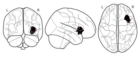
Another GRU model with the same architecture, but slightly different hyperparameters, was trained using segments only from the right Insula instead of whole brain. Following are the results.
4.1. Search Grid With 5-fold Cross Validation
The model was fine tuned by finding optimal values for the following hyperparmeters:1) L2 regularization and 2) dropout rate applied to each of the hidden layers, and 3) learning_rate of the Adam optimizer.
Optimal hyperparameters were found by doing a full grid-search over 20 combinations of hyperparameteres, and cross-validating each combination with a nested 5-fold cross-validation method. A total of 20 models were trained and validated. Following plot shows the performance of each model in terms of its training and validation accuracies. The models are shown in the descending order of their mean validation accuracy. The error bars indicate standard deviation across folds.
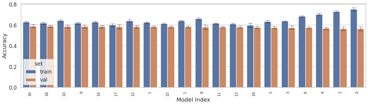
Best performing model yielded mean training and validation accuracies of 0.63 and 0.59, respectively. Its hyperparameters were: 1) L2 = 0.003, dropout = 0.3, and learning_rate = 0.006.
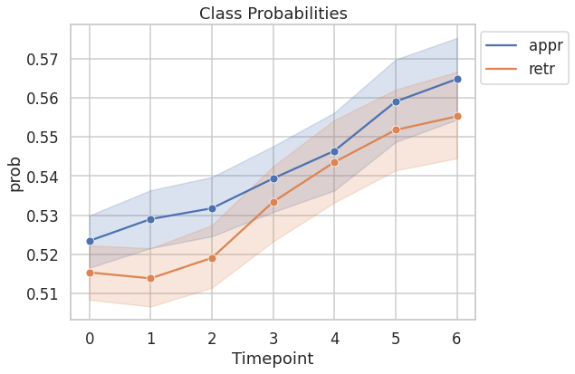
4.2. Probability of predicting the true class as a function of time
Following figure shows probability of predicting the true class as a function of time. The probability of predicting the true class increases with time.
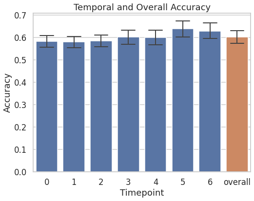
4.3. Test Accuracy
The trained model was tested on the near-miss segments of the 19 held-out participants. Following figure shows temporal and overall accuracies on the held-out participants. The model performs resonably well from the 1st timepoint (TP) itself, with a mean accuracy of 0.58. The mean accuracy steadily increases to 0.63 by the 7th TP. “Overall” accuracy is the mean accuracy across TP, which is 0.603.
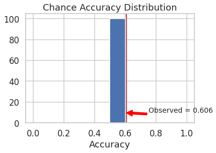
4.4. Chance Accuracy
To assess significance of the model performance, the observed test accuracy was compared against the accuracy that would be observed if the model was to guess one of the two classes at random. To that end, model with the best hyperparameter settings was trained on the training set a hundred times, each time with randomly shuffled labels. At every iteration, the model was tested on the test set with “non-shuffled” (i.e., true) labels. This process was meant to simulate a chance accuracy distribution. The mean of the chance accuracy distribution formed the baseline performance measure against the observed performance of the model when trained on true labels. The observed test accuracy was significantly greater than the average chance accuracy (p < 0.009). See the figure below.
Accuracy
Observed: 0.61
Chance: 0.50
Observed > Chance (p = 0.0099)
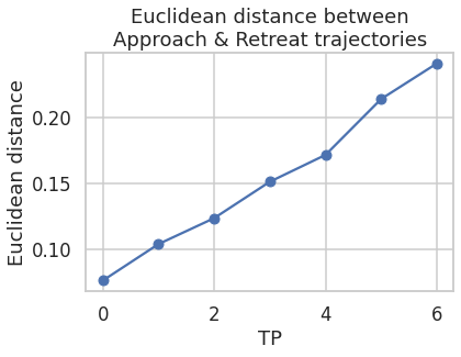
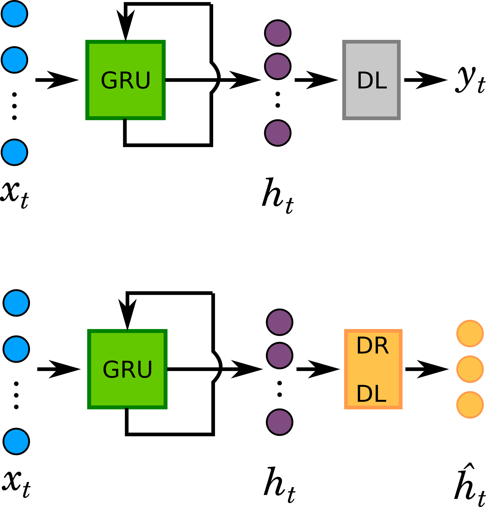
4.5. Temporal Trajectories
GRU outputs hidden states that are typically high dimensional. Hidden states (\(h_{t}\)) capture spatio-temporal variance that is most useful in maintaning class separability. To visualize dynamics, \(h_{t}\) was linearly projected onto a lower (3D) dimensional space, \(\hat{h_{t}}\). This was done by replacing the output layer with a Dimensionality Reduction Dense Layer (DRDL) with three linear units. In essence, this is a supervised non-linear dimensional reduction step.
The 3-dimensional representations of \(h_{t}\) (\(\hat{h_{t}}\)) for both stimulus class are plotted along the three axes of the coordinate system below. The plot represents the temporal trajectories of the two classes. At the first timepoint the two classes are closest to each other. Distance between them increases with every timepoint. Next plot shows the Euclidean distance between the two classes as a function of time.