from IPython.display import HTML

HTML('''<script>
code_show=true;
function code_toggle() {
 if (code_show){
 $('div.input').hide();
 } else {
 $('div.input').show();
 }
 code_show = !code_show
}
$( document ).ready(code_toggle);
</script>
<form action="javascript:code_toggle()"><input type="submit" value="Show Code"></form>''')
3. Statistical Data Analysis
# Import useful libraries
import pandas as pd
import numpy as np
import pickle
import matplotlib.pyplot as plt

from collections import defaultdict

import matplotlib as mpl
import seaborn as sns
sns.set(style ='white',font_scale=1.25)
%matplotlib inline

# Import all functions
from functions import *

# Set waring to 'ignore' to prevent them from prining on screen
import warnings
warnings.filterwarnings('ignore')
with open('data/wrangled_data.pkl','rb') as file:
    housing_orig, FEATURES,transformers = pickle.load(file)
print('Dimensions of the dataset',housing_orig[FEATURES['num']+FEATURES['cat']+FEATURES['aug_num']].shape)
Dimensions of the dataset (1454, 85)
housing = housing_orig.copy()
housing.head()
y = housing.SalePrice
3.1. Numerical Features
housing_num = housing[FEATURES['num']+FEATURES['aug_num']]
3.1.1. Correlation amongst Numerical Features
plt.figure(figsize=(20,20))
sns.heatmap(housing_num.corr(method='spearman'),
            vmax=1,vmin=-1,annot=True,
            cmap='coolwarm',
            fmt='.2f',annot_kws={'size':8})
_=plt.title("Feature correlation matrix")
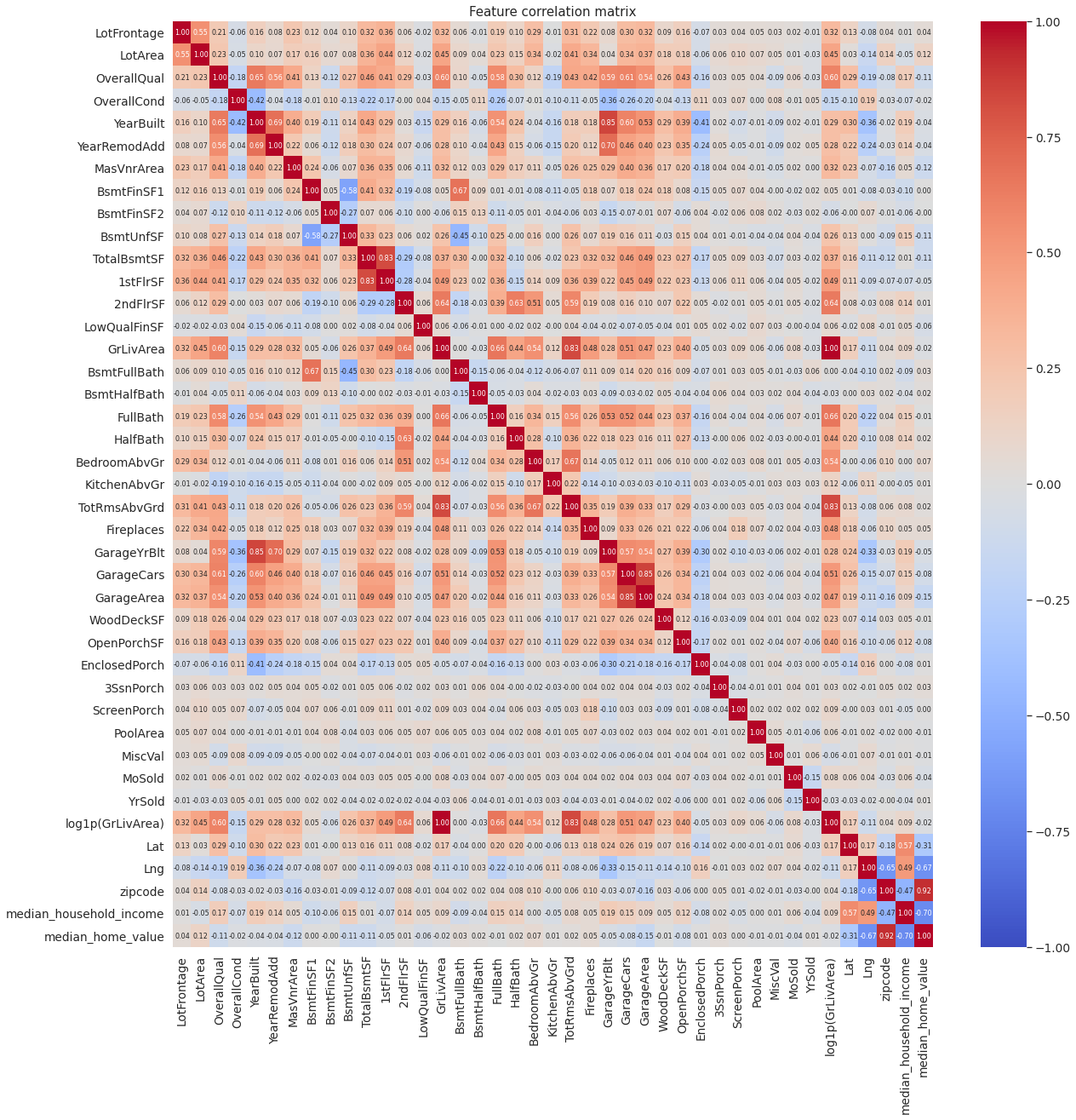
Several numerical features are highly correlated with one another. Highest positive correlation is between house and garage year built (YearBuilt and GarageYrBlt). This is not unexpected, as most house garages are built along with the house itself. A new feature called GarageYrBltMinusYearBuilt is created, which models the difference between the year in which the garage and the house was built.
Second highest positive correlation is between total number of rooms (TotRmsAbvGrd) and log of total square feet area above ground (log1p(GrLivArea)). Its highly likely that TotRmsAbvGrd is highly correlated with GrLivArea itself. This is expected as houses with greater area tend to have more number of rooms. A new feature called AreaPerRoom is added, which models the average area per room by dividing the TotRmsAbvGrd by GrLivArea.
Let’s check the correlation matrix again.
from sklearn.preprocessing import FunctionTransformer

def addFeatures(X, new_features=['AreaPerRoom','GarageYrBltMinusYearBuilt']):
    for feat in new_features:
        if feat == 'AreaPerRoom':
            #GrLivArea = np.expm1(X['log1p(GrLivArea)'])
            X['AreaPerRoom'] = X['GrLivArea'].divide(X.TotRmsAbvGrd)
            X['log1p(AreaPerRoom)'] = np.log1p(X.AreaPerRoom)
        elif feat == 'GarageYrBltMinusYearBuilt':
            X['GarageYrBltMinusYearBuilt']=X['GarageYrBlt'].subtract(X.YearBuilt)
    return X

feature_adder = FunctionTransformer(addFeatures,validate=False,kw_args=dict(new_features =['AreaPerRoom','GarageYrBltMinusYearBuilt']))
transformers.append(('feature_adder',feature_adder))
housing = feature_adder.fit_transform(housing)
#GrLivArea = np.expm1(housing_num['log1p(GrLivArea)'])
housing_num['AreaPerRoom'] = housing_num['GrLivArea'].divide(housing_num.TotRmsAbvGrd)
housing_num['log1p(AreaPerRoom)'] = np.log1p(housing_num['AreaPerRoom'])
housing_num['GarageYrBltMinusYearBuilt'] = housing_num['GarageYrBlt'].subtract(housing_num.YearBuilt)

# Add the engineered features
FEATURES['eng_num'].extend(['AreaPerRoom','log1p(AreaPerRoom)','GarageYrBltMinusYearBuilt'])
housing_num.equals(housing[FEATURES['num']+FEATURES['aug_num']+FEATURES['eng_num']])
True
plt.figure(figsize=(20,20))
sns.heatmap(housing_num.corr(method='spearman'),
            vmax=1,vmin=-1,annot=True,
            cmap='coolwarm',
            fmt='.2f',annot_kws={'size':8})
_=plt.title("Feature correlation matrix after adding two new features")
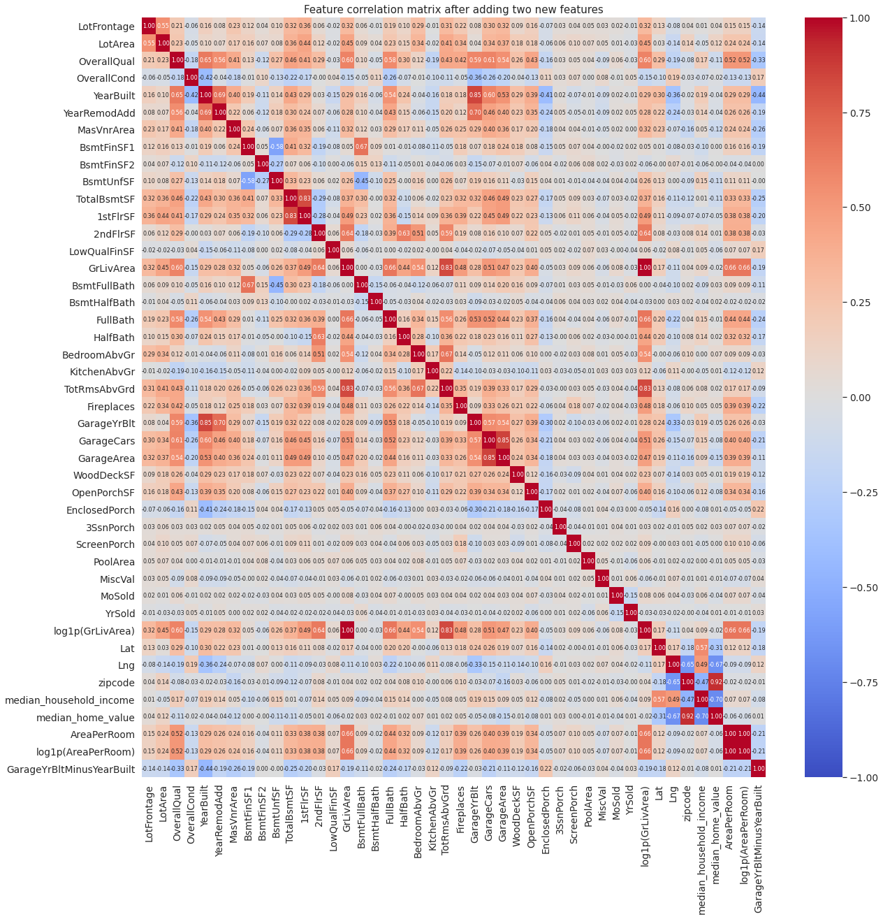
Unlike the parent features, the newly added features (AreaPerRoom and GarageYrBltMinusYearBuilt) are not that highly correlated with the rest of the features. Neither are they highly correlated with the parent features.
3.1.2. Correlation with Sale Price
housing_num.corrwith(y,method='spearman').sort_values(ascending=True).plot.barh(figsize=(8,10),title = 'Spearman correaltion with Sale Price')
plt.axvline(x=0.4,linestyle='--',color='r')
plt.axvline(x=-0.4,linestyle='--',color='r')
<matplotlib.lines.Line2D at 0x7fddb8960160>
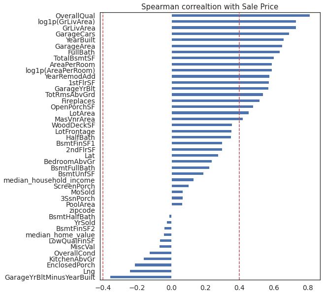
Several features are highly correlated (> 0.4) with the sale price. One of the engineered (newly added) features, AreaPerRoom, is also highly correlated (~0.6) with the sale price. In fact, it is more correlated than one of its parent features from which it is derived (TotRmsAbvGrd). GarageYrBlitMinusYearBuilt is another engineered feature. It has the highest negative correlation with the sale price. Both engineered features are candidates for predicting the sale price.
Comments/Observation:
Following numercial features showed strong positve correlation (>= 0.4) with the sale price (listed in descending order of their correlation strength with sale price).
Overall Quality (OverallQual)
Above grade living area in sq. ft. (GrLivArea)
Total garage car capacity in number of cars (GarageCars)
Year built (YrBuilt)
Garage area in sq.ft (GarageArea)
Number of full bathrooms above grade (FullBath)
Total area of the basement in sq. ft. (TotalBsmtSF)
Average size of a room in sq. ft. (AreaPerRoom)
Year when the house of remodeled (YearRemodAdd)
Garage year built (GarageYrBlt)
Area of the first floor in sq. ft.(1stFlrSF)
Total rooms above grade (TotRmsAbvGrd)
Number of fireplaces (FirePlaces)
Open porch area in sq. ft. (OpenPorchSF)
Lot Area in sq. ft. (LotArea)
Masonry veneer area in sq, ft. (MasVnrArea)
3.2. Categorical Features
3.2.1. Non-parametric ANOVA
import scipy.stats as stats
housing_cat = housing[FEATURES['cat']]
def anova(frame):
    anv = pd.DataFrame()
    anv['feature'] = frame.drop('SalePrice',axis=1).columns
    pvals = []
    for c in frame.drop('SalePrice',axis=1).columns:
        samples = []
        for cls in frame[c].unique():
            s = frame[frame[c] == cls]['SalePrice'].values
            samples.append(s)
        pval = stats.kruskal(*samples)[1]
        pvals.append(pval)
    anv['pval'] = pvals
    return anv.sort_values('pval').reset_index(drop=True)

a = anova(housing_cat.join(housing.SalePrice))
a['disparity'] = np.log(1./a['pval'].values)
plt.figure(figsize=(8,10))
sns.barplot(x='disparity',y='feature',data=a,color=sns.color_palette(n_colors=1)[0])
x=plt.xticks(rotation=90)
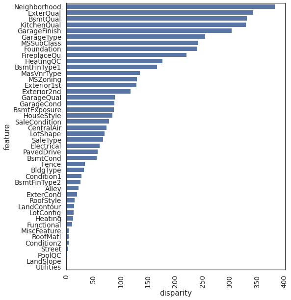
The above bar plot shows influence of each categorical feature on the sale price. Features with higher disparity have greater influence on the sale price.
3.2.2. Ordinal Features
Description of following categorical feature indicate they have ordinal categories
LandSlope
ExterQual
ExterCond
BsmtQual
BsmtCond
BsmtExposure
BsmtFinType1
BsmtFinType2
HeatingQC
KitchenQual
FireplaceQu
GarageFinish
GarageQual
GarageCond
PavedDrive
PoolQC
ordinal_map = {'LandSlope':{'Gtl':0.,'Mod':1.,'Sev':2.},
               'ExterQual':{'Ex':4.,'Gd':3.,'TA':2.,'Fa':1.,'Po':0.},
               'ExterCond':{'Ex':4.,'Gd':3.,'TA':2.,'Fa':1.,'Po':0.},
               'BsmtQual':{'Ex':5.,'Gd':4.,'TA':3.,'Fa':2.,'Po':1.,'Missing':0.}, # Houses that don't have a basement are assigned Typical/Average rating
               'BsmtCond':{'Gd':4., 'TA':3., 'Fa':2., 'Po':1.,'Missing':0.},
               'BsmtExposure':{'Gd':4.,'Av':3.,'Mn':2.,'No':1.,'Missing':0.},
               'BsmtFinType1': {'Missing': 0.,'Unf':1.,'LwQ':2.,'Rec':3.,'BLQ':4.,'ALQ':5.,'GLQ':6.},
               'BsmtFinType2': {'Missing': 0.,'Unf':1.,'LwQ':2.,'Rec':3.,'BLQ':4.,'ALQ':5.,'GLQ':6.},
               'HeatingQC':{'Po':0.,'Fa':1.,'TA':2.,'Gd':3.,'Ex':4.},
               'KitchenQual':{'Ex':5.,'Gd':4.,'TA':3.,'Fa':2.,'Po':1.,'Missing':0},
               'FireplaceQu':{'Ex':5.,'Gd':4.,'TA':3.,'Fa':2.,'Po':1.,'Missing':0.},
               'GarageFinish':{'Fin':3., 'RFn':2., 'Unf':1., 'Missing':0.},
               'GarageQual':{'Ex':5., 'Gd':4., 'TA':3., 'Fa':2., 'Po':1., 'Missing':0.},
               'GarageCond':{'Ex':5., 'Gd':4., 'TA':3., 'Fa':2., 'Po':1., 'Missing':0.},
               'PavedDrive':{'Y':2., 'P':1., 'N':0.},
               'PoolQC':{'Ex':4., 'Gd':3., 'TA':2., 'Fa':1., 'Missing':0.}}

## Add ordinal features to FEATURES
FEATURES['ord_num'].extend(list(ordinal_map.keys()))
FEATURES.keys()
dict_keys(['cat', 'num', 'aug_num', 'eng_num', 'ord_num'])
def LabelEncode(X,mapper=ordinal_map):
    return X.replace(mapper)

LabelEncoder = FunctionTransformer(LabelEncode,validate=False,kw_args=dict(mapper=ordinal_map))
transformers.append(('LabelEncoder',LabelEncoder))

housing_cat = LabelEncoder.fit_transform(housing_cat)
housing = LabelEncoder.fit_transform(housing)
housing_cat[FEATURES['ord_num']].equals(housing[FEATURES['ord_num']])
True
housing[FEATURES['ord_num']].info()
<class 'pandas.core.frame.DataFrame'>
Int64Index: 1454 entries, 1 to 1460
Data columns (total 16 columns):
 #   Column        Non-Null Count  Dtype
---  ------        --------------  -----
 0   LandSlope     1454 non-null   float64
 1   ExterQual     1454 non-null   float64
 2   ExterCond     1454 non-null   float64
 3   BsmtQual      1454 non-null   float64
 4   BsmtCond      1454 non-null   float64
 5   BsmtExposure  1454 non-null   float64
 6   BsmtFinType1  1454 non-null   float64
 7   BsmtFinType2  1454 non-null   float64
 8   HeatingQC     1454 non-null   float64
 9   KitchenQual   1454 non-null   float64
 10  FireplaceQu   1454 non-null   float64
 11  GarageFinish  1454 non-null   float64
 12  GarageQual    1454 non-null   float64
 13  GarageCond    1454 non-null   float64
 14  PavedDrive    1454 non-null   float64
 15  PoolQC        1454 non-null   float64
dtypes: float64(16)
memory usage: 233.1 KB
Note: From here train and test sets are processed togather
from sklearn.pipeline import Pipeline

train_raw = pd.read_csv('data/train.csv',index_col='Id')
test_raw = pd.read_csv('data/test.csv',index_col='Id')
my_pipeline = Pipeline(transformers)
my_pipeline.fit(train_raw)
train = my_pipeline.transform(train_raw)

print('Manually and pipeline created datasets are equal:')
print(housing.drop('log1p(SalePrice)',axis=1).equals(train))

test = my_pipeline.transform(test_raw)
Manually and pipeline created datasets are equal:
True
train_raw.shape
(1460, 80)
train.shape
(1454, 89)
3.2.3. One hot ecoding: one hot encode following features
MSSubClass
MSZoning
Street
Alley
LotShape
LandContour
Utilities
LotConfig
Neighborhood
Condition1
Condition2
BldgType
HouseStyle
RoofStyle
RoofMatl
Exterior1st
Exterior2nd
MasVnrType
Foundation
Heating
CentralAir
Electrical
Functional
GarageType
Fence
MiscFeature
SaleType
SaleCondition
## Add onehot_cat features to FEATURES
FEATURES['onehot_cat'].extend([cat for cat in FEATURES['cat'] if cat not in FEATURES['ord_num']])
FEATURES.keys()
dict_keys(['cat', 'num', 'aug_num', 'eng_num', 'ord_num', 'onehot_cat'])
train_test_cat = pd.concat([train[FEATURES['onehot_cat']],test[FEATURES['onehot_cat']]])
train_test_cat = pd.get_dummies(train_test_cat,drop_first=True)
train = pd.concat([train,train_test_cat.loc[train.index,:]],axis=1)
train.drop(FEATURES['onehot_cat'],axis=1,inplace=True)

test = pd.concat([test,train_test_cat.loc[test.index,:]],axis=1)
test.drop(FEATURES['onehot_cat'],axis=1,inplace=True)

y = np.log1p(train['SalePrice'])
train.drop('SalePrice',axis=1,inplace=True)
print('Training set size:',train.shape)
Training set size: (1454, 240)
print('Test set size:',test.shape)
Test set size: (1459, 240)
3.3. Interactions
Check pairwise feature correlations
Create interactions of feature pairs with high correlations (> 0.4)
#corr_df = train.drop(['ExterQual','KitchenQual'],axis=1).corr()
corr_df = train.corr()
''' Create a dictionary with feature pairs as keys and their correlations as values'''
corr_dict = {}
for key, val in corr_df.unstack().to_dict().items():
    if (key == key[::-1]) or (key in corr_dict) or (key[::-1] in corr_dict):
        pass
    else:
        corr_dict[key] = val
'''Find feature pairs with corr > 0.4'''
high_corr_dict = {}
targetCorr = 0.4
for key, val in corr_dict.items():
    if val > targetCorr:
        high_corr_dict[key] = val

print('Total pairs with corr greater than %.2f: %i' %(targetCorr,len(high_corr_dict)))

'''Sort corr dict in descending order'''
from collections import OrderedDict
high_corr_dict = OrderedDict(sorted(high_corr_dict.items(), key=lambda x: x[1],reverse=True))
#print(high_corr_dict)
Total pairs with corr greater than 0.40: 226
num_feats = FEATURES['num'] + FEATURES['aug_num'] + FEATURES['eng_num'] + FEATURES['ord_num']
for feat1, feat2 in high_corr_dict:
    if (feat1 in num_feats) or (feat2 in num_feats):
        FEATURES['interactions_num'].append('X'.join([feat1,feat2]))
    else:
        FEATURES['interactions'].append('X'.join([feat1,feat2]))
    train['X'.join([feat1,feat2])] = train[feat1] * train[feat2]
    test['X'.join([feat1,feat2])] = test[feat1] * test[feat2]
print("Total number of training examples : " + str(train.shape[0]))
print("Total number of training features : " + str(train.shape[1]))
print("-"*50)
print("Total number of test examples : " + str(test.shape[0]))
print("Total number of test features : " + str(test.shape[1]))
Total number of training examples : 1454
Total number of training features : 466
--------------------------------------------------
Total number of test examples : 1459
Total number of test features : 466
with open('data/processed_data.pkl','wb') as file:
    pickle.dump((train,y,test,FEATURES),file)