from IPython.display import HTML

HTML('''<script>
code_show=true;
function code_toggle() {
 if (code_show){
 $('div.input').hide();
 } else {
 $('div.input').show();
 }
 code_show = !code_show
}
$( document ).ready(code_toggle);
</script>
<form action="javascript:code_toggle()"><input type="submit" value="Show Code"></form>''')
1. Data Wrangling
Problem Statement
Buying a house can be a very challenging process. It takes time, patience, and a lot of research to find a house that you like and then negotiate the right price for it. There are several features that influence house price such as the building type, total number of rooms, garage size, masonary work, location, utilities, and many more. Can house price be estimated (or predicted) using these features? Can we identify features that influence house price the most? How important is Building Type in determining the price? What influences the price more: location or size (sq.ft.)? How much value does remodeling add to the house? These are a few questions among many more that I intend to explore and answer.
Dataset
Dataset is available on kaggle (https://www.kaggle.com/c/house-prices-advanced-regression-techniques). It is the Ames Housing dataset, compiled by Dean De Cock. It has 1460 instances and 79 explanatory variables that describe almost every aspect of residential homes in Ames, Iowa.
In this part, we will explore the data. In the process, we will clean and augment the data with additional information from other sources. We will perform the following steps:
Identify and remove outliers
Fill missing values
Augment the dataset by collecting and adding data from other sources like Google’s Geocoding API and uszipcode library
# Import useful libraries
import pandas as pd
import numpy as np
import pickle
import matplotlib.pyplot as plt

import matplotlib as mpl
import seaborn as sns
%matplotlib inline

sns.set(style ='white',font_scale=1.25)

# sklearn pipeline tools
from sklearn.compose import ColumnTransformer
from sklearn.pipeline import Pipeline

# Set waring to 'ignore' to prevent them from prining on screen
import warnings
warnings.filterwarnings('ignore')
# Load the dataset, and look at first few rows
housing_raw = pd.read_csv('data/train.csv',index_col='Id')
housing = housing_raw.copy()
housing.head()
| MSSubClass | MSZoning | LotFrontage | LotArea | Street | Alley | LotShape | LandContour | Utilities | LotConfig | ... | PoolArea | PoolQC | Fence | MiscFeature | MiscVal | MoSold | YrSold | SaleType | SaleCondition | SalePrice | |
|---|---|---|---|---|---|---|---|---|---|---|---|---|---|---|---|---|---|---|---|---|---|
| Id | |||||||||||||||||||||
| 1 | 60 | RL | 65.0 | 8450 | Pave | NaN | Reg | Lvl | AllPub | Inside | ... | 0 | NaN | NaN | NaN | 0 | 2 | 2008 | WD | Normal | 208500 |
| 2 | 20 | RL | 80.0 | 9600 | Pave | NaN | Reg | Lvl | AllPub | FR2 | ... | 0 | NaN | NaN | NaN | 0 | 5 | 2007 | WD | Normal | 181500 |
| 3 | 60 | RL | 68.0 | 11250 | Pave | NaN | IR1 | Lvl | AllPub | Inside | ... | 0 | NaN | NaN | NaN | 0 | 9 | 2008 | WD | Normal | 223500 |
| 4 | 70 | RL | 60.0 | 9550 | Pave | NaN | IR1 | Lvl | AllPub | Corner | ... | 0 | NaN | NaN | NaN | 0 | 2 | 2006 | WD | Abnorml | 140000 |
| 5 | 60 | RL | 84.0 | 14260 | Pave | NaN | IR1 | Lvl | AllPub | FR2 | ... | 0 | NaN | NaN | NaN | 0 | 12 | 2008 | WD | Normal | 250000 |
5 rows × 80 columns
# Datatype of each column
housing.info()
<class 'pandas.core.frame.DataFrame'>
Int64Index: 1460 entries, 1 to 1460
Data columns (total 80 columns):
 #   Column         Non-Null Count  Dtype
---  ------         --------------  -----
 0   MSSubClass     1460 non-null   int64
 1   MSZoning       1460 non-null   object
 2   LotFrontage    1201 non-null   float64
 3   LotArea        1460 non-null   int64
 4   Street         1460 non-null   object
 5   Alley          91 non-null     object
 6   LotShape       1460 non-null   object
 7   LandContour    1460 non-null   object
 8   Utilities      1460 non-null   object
 9   LotConfig      1460 non-null   object
 10  LandSlope      1460 non-null   object
 11  Neighborhood   1460 non-null   object
 12  Condition1     1460 non-null   object
 13  Condition2     1460 non-null   object
 14  BldgType       1460 non-null   object
 15  HouseStyle     1460 non-null   object
 16  OverallQual    1460 non-null   int64
 17  OverallCond    1460 non-null   int64
 18  YearBuilt      1460 non-null   int64
 19  YearRemodAdd   1460 non-null   int64
 20  RoofStyle      1460 non-null   object
 21  RoofMatl       1460 non-null   object
 22  Exterior1st    1460 non-null   object
 23  Exterior2nd    1460 non-null   object
 24  MasVnrType     1452 non-null   object
 25  MasVnrArea     1452 non-null   float64
 26  ExterQual      1460 non-null   object
 27  ExterCond      1460 non-null   object
 28  Foundation     1460 non-null   object
 29  BsmtQual       1423 non-null   object
 30  BsmtCond       1423 non-null   object
 31  BsmtExposure   1422 non-null   object
 32  BsmtFinType1   1423 non-null   object
 33  BsmtFinSF1     1460 non-null   int64
 34  BsmtFinType2   1422 non-null   object
 35  BsmtFinSF2     1460 non-null   int64
 36  BsmtUnfSF      1460 non-null   int64
 37  TotalBsmtSF    1460 non-null   int64
 38  Heating        1460 non-null   object
 39  HeatingQC      1460 non-null   object
 40  CentralAir     1460 non-null   object
 41  Electrical     1459 non-null   object
 42  1stFlrSF       1460 non-null   int64
 43  2ndFlrSF       1460 non-null   int64
 44  LowQualFinSF   1460 non-null   int64
 45  GrLivArea      1460 non-null   int64
 46  BsmtFullBath   1460 non-null   int64
 47  BsmtHalfBath   1460 non-null   int64
 48  FullBath       1460 non-null   int64
 49  HalfBath       1460 non-null   int64
 50  BedroomAbvGr   1460 non-null   int64
 51  KitchenAbvGr   1460 non-null   int64
 52  KitchenQual    1460 non-null   object
 53  TotRmsAbvGrd   1460 non-null   int64
 54  Functional     1460 non-null   object
 55  Fireplaces     1460 non-null   int64
 56  FireplaceQu    770 non-null    object
 57  GarageType     1379 non-null   object
 58  GarageYrBlt    1379 non-null   float64
 59  GarageFinish   1379 non-null   object
 60  GarageCars     1460 non-null   int64
 61  GarageArea     1460 non-null   int64
 62  GarageQual     1379 non-null   object
 63  GarageCond     1379 non-null   object
 64  PavedDrive     1460 non-null   object
 65  WoodDeckSF     1460 non-null   int64
 66  OpenPorchSF    1460 non-null   int64
 67  EnclosedPorch  1460 non-null   int64
 68  3SsnPorch      1460 non-null   int64
 69  ScreenPorch    1460 non-null   int64
 70  PoolArea       1460 non-null   int64
 71  PoolQC         7 non-null      object
 72  Fence          281 non-null    object
 73  MiscFeature    54 non-null     object
 74  MiscVal        1460 non-null   int64
 75  MoSold         1460 non-null   int64
 76  YrSold         1460 non-null   int64
 77  SaleType       1460 non-null   object
 78  SaleCondition  1460 non-null   object
 79  SalePrice      1460 non-null   int64
dtypes: float64(3), int64(34), object(43)
memory usage: 923.9+ KB
We can see there are a lot of numerical and categorical features.
Lets first take look at the numerical (particularly continous) features to spot outliers.
# Created a list of continous features to check their distribution and spot potential outliers
cont_feats = ['SalePrice','LotFrontage',
              'LotArea','MasVnrArea',
              'BsmtFinSF1','BsmtFinSF2',
              'BsmtUnfSF','TotalBsmtSF',
              '1stFlrSF','2ndFlrSF',
              'LowQualFinSF','GrLivArea',
              'GarageArea','WoodDeckSF',
              'OpenPorchSF','EnclosedPorch',
              'ScreenPorch']
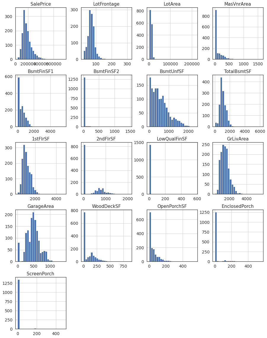
1.1. Distributions of Continous Features.
_=housing[cont_feats].hist(figsize = (15,20),bins=25)
1.2. Distribution of SalePrice (target variable)
from scipy import stats
sns.distplot(housing.SalePrice, kde=False, bins=30)
plt.text(x=5e5, y=100,s='Skew = %.3f' %(housing.SalePrice.skew()),fontdict={'fontsize':14})
_=plt.xticks(rotation = 45)
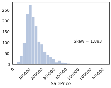
Distribution has a postive skew. Let apply a log tranform.
housing['log1p(SalePrice)'] = np.log1p(housing['SalePrice'])
plt.figure(figsize=(15,5))
plt.subplot(1,2,1)
sns.distplot(housing.SalePrice, kde=False, bins=30)
plt.text(x=5e5, y=100,s='Skew = %.3f' %(housing.SalePrice.skew()),fontdict={'fontsize':14})
_=plt.xticks(rotation = 45)

plt.subplot(1,2,2)
sns.distplot(housing['log1p(SalePrice)'], kde=False, bins=30)
_=plt.text(x=12.5, y=150,s='Skew = %.3f' %(housing['log1p(SalePrice)'].skew()),fontdict={'fontsize':14})
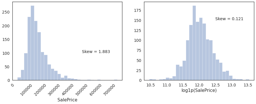
Looks close to normal after tranforming.
1.3. Outlier Identification
1.3.1. Distribution of GrLivArea
sns.distplot(housing.GrLivArea, kde=False, bins=30)
plt.text(x=3000, y=150,s='Skew = %.3f' %(housing.GrLivArea.skew()),fontdict={'fontsize':14})
_=plt.xticks(rotation = 45)
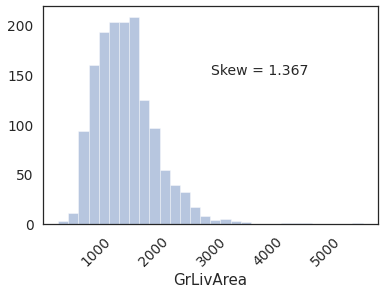
Distribution has positve skew.
Lets also apply log tranform to GrLivArea.
# Initialize a transformer list object to keep track of all data preprocessing steps
transformers = []
def log1p(X,columns):
    X_new = X.copy()
    for col in columns:
        X_new['log1p({})'.format(col)] = np.log1p(X_new[col])
        #X_new.drop(col,axis=1,inplace=True)
    return X_new

from sklearn.preprocessing import FunctionTransformer
log_trans = FunctionTransformer(log1p,validate=False,
                                      kw_args=dict(columns=['GrLivArea']))
transformers.append(('log_trans',log_trans))
housing['log1p(GrLivArea)'] = np.log1p(housing.GrLivArea)
plt.figure(figsize=(15,5))
plt.subplot(1,2,1)
sns.distplot(housing['log1p(GrLivArea)'],kde=False,bins=int(np.sqrt(len(housing))))
plt.text(x=6, y=120,s='Skew = %.3f' %(housing['log1p(GrLivArea)'].skew()),fontdict={'fontsize':14})
plt.subplot(1,2,2)
plt.scatter(housing['log1p(GrLivArea)'], housing['log1p(SalePrice)'], c='blue',marker = 's',alpha=0.25)
plt.xlabel('log1p(GrLivArea)')
plt.ylabel('log1p(SalePrice)')
Text(0, 0.5, 'log1p(SalePrice)')
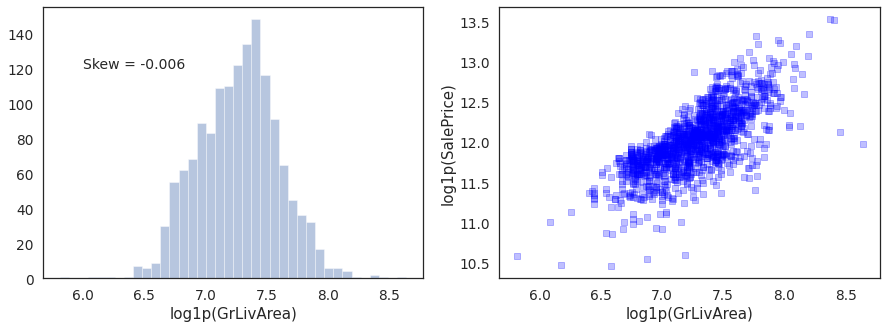
No apparent outliers in log of GrLivArea. Distrubution also looks normal.
1.3.2. Distribution of GarageArea
sns.distplot(housing.GarageArea, kde=False, bins=30)
plt.text(x=1000, y=150,s='Skew = %.3f' %(housing.GarageArea.skew()),fontdict={'fontsize':14})
_=plt.xticks(rotation = 45)
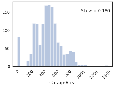
Distibution looks reasonably normal.
plt.scatter(housing.GarageArea,
            housing.SalePrice, c='blue',marker = 's',alpha=0.25)
plt.xlabel('GarageArea')
plt.ylabel('SalePrice')
Text(0, 0.5, 'SalePrice')
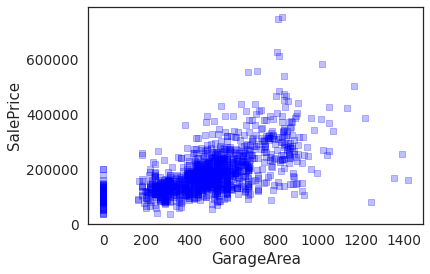
No apparent outliers in the scatter plot
1.3.3. Distribution LotArea
sns.distplot(housing.LotArea, kde=False, bins=50)
plt.text(x=50000, y=150,s='Skew = %.3f' %(housing.LotArea.skew()),fontdict={'fontsize':14})
_=plt.xticks(rotation = 45)
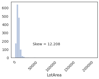
Distribution is highly skewed due to outliers.
plt.scatter(housing.LotArea,
            housing['log1p(SalePrice)'], c='blue',marker = 's',alpha=0.25)
plt.axvline(x=60000,color='red',linestyle='--')
plt.xlabel('LotArea')
plt.ylabel('log1p(SalePrice)')
Text(0, 0.5, 'log1p(SalePrice)')
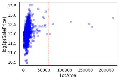
LotArea > 60000 seem like outliers. Lets remove them.
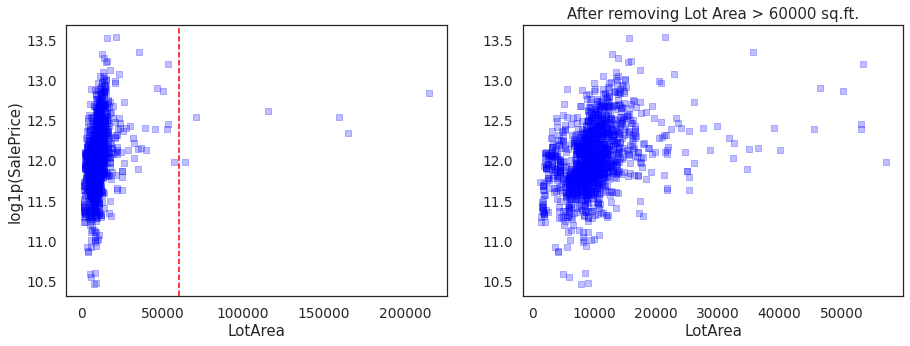
plt.figure(figsize=(15,5))
plt.subplot(1,2,1)
plt.scatter(housing.LotArea,
            housing['log1p(SalePrice)'],
            c='blue',marker = 's',alpha=0.25)
plt.axvline(x=60000,color='red',linestyle='--')
plt.xlabel('LotArea')
plt.ylabel('log1p(SalePrice)')

outlier = pd.DataFrame()
outlier['LotArea'] = housing.LotArea > 60000

plt.subplot(1,2,2)
plt.scatter(housing[~outlier.any(axis=1)].LotArea, housing[~outlier.any(axis=1)]['log1p(SalePrice)'], c='blue',marker = 's',alpha=0.25)
plt.xlabel('LotArea')
plt.ylabel('')
plt.title('After removing Lot Area > %.0f sq.ft.' %(60000))
Text(0.5, 1.0, 'After removing Lot Area > 60000 sq.ft.')
plt.figure(figsize=(15,5))
plt.subplot(1,2,1)
sns.distplot(housing.LotArea, kde=False, bins=50)
plt.text(x=50000, y=150,s='Skew = %.3f' %(housing.LotArea.skew()),fontdict={'fontsize':14})
_=plt.xticks(rotation = 45)
_=plt.title('Before outlier removal')

plt.subplot(1,2,2)
sns.distplot(housing[~outlier.any(axis=1)]['LotArea'], kde=False, bins=50)
plt.text(x=15000, y=100,s='Skew = %.3f' %(housing[~outlier.any(axis=1)]['LotArea'].skew()),fontdict={'fontsize':14})
_=plt.title('After outlier removal')
_=plt.xticks(rotation = 45)
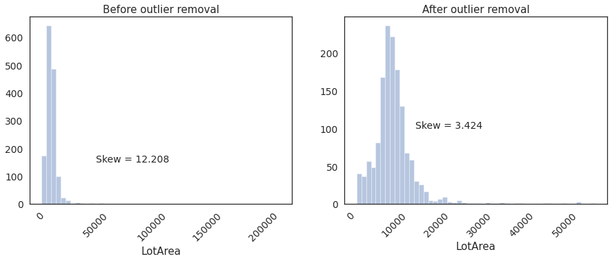
Skeweness improved considerably after removing outliers. Distribution has looks reasonably normal.
print('Number of examples before outlier removal: ',housing.shape[0])
print('Number of examples after outlier removal: ',housing[~outlier.any(axis=1)].shape[0])
print('%i examples are excluded' %(housing.shape[0]-housing[~outlier.any(axis=1)].shape[0]))
Number of examples before outlier removal:  1460
Number of examples after outlier removal:  1454
6 examples are excluded
def remove_outliers(X,columns,thresholds):
    outlier = pd.DataFrame()
    for column,threshold in zip(columns,thresholds):
        if column == 'GrLivArea':
            outlier[column] = X[column] > threshold
        elif column == 'LotArea':
            percentile = np.percentile(X[column],99)
            outlier[column] = X[column] > threshold
        else:
            print(column+' not processed for outliers')
    return X[~outlier.any(axis=1)]

outlier_remover = FunctionTransformer(remove_outliers,validate=False,
                                      kw_args=dict(columns=['LotArea'],
                                                   thresholds=[60000]))
outlier_remover.fit(housing) # Fit on training data

transformers.append(('outlier_remover',outlier_remover))

housing = outlier_remover.transform(housing) ## Use this line instead the next cell
#housing = housing[~outlier.any(axis=1)]
print('Dataset size:',housing.shape)
Dataset size: (1454, 82)
For more advanced methods of dealing with outliers, ref to:
1. https://pyod.readthedocs.io/en/latest/
2. https://scikit-learn.org/stable/modules/generated/sklearn.ensemble.IsolationForest.html#sklearn.ensemble.IsolationForest
In the next step we will treat missing values.
1.4. Missing Value Treatment
1.4.1. Categorical Features
Lets first treat missing values in the categorical features
MSSubclass is a categorical feature but it got loaded as a numerical feature, so lets change it to categorical.
def to_str(X,columns):
    for column in columns:
        X[column] = X[column].astype(str)
    return X

to_string = FunctionTransformer(to_str,validate=False,
                                      kw_args=dict(columns=["MSSubClass"]))
to_string.fit(housing) # fit on training data
transformers.append(('MSSubClass_to_str',to_string))
housing = to_string.transform(housing)
from collections import defaultdict

# Initialize a feature dictionary which will keep track of all features
FEATURES = defaultdict(list)
missing_vals_cat = pd.DataFrame(columns=['Feature', '# of missing vals','% of missing vals'])
for feature, numNan in housing.isnull().sum().iteritems():
    if housing[feature].dtypes == 'object':
        FEATURES['cat'].append(feature)
        if numNan != 0:
            missing_vals_cat = pd.concat([missing_vals_cat,pd.DataFrame([feature,numNan,(numNan/housing.shape[0])*100],
                                                                        index=['Feature', '# of missing vals','% of missing vals']).T])

missing_vals_cat.sort_values(by=['% of missing vals'],ascending=False).reset_index(drop=True)
| Feature | # of missing vals | % of missing vals | |
|---|---|---|---|
| 0 | PoolQC | 1448 | 99.5873 |
| 1 | MiscFeature | 1402 | 96.4237 |
| 2 | Alley | 1363 | 93.7414 |
| 3 | Fence | 1173 | 80.674 |
| 4 | FireplaceQu | 690 | 47.4553 |
| 5 | GarageType | 81 | 5.57084 |
| 6 | GarageFinish | 81 | 5.57084 |
| 7 | GarageQual | 81 | 5.57084 |
| 8 | GarageCond | 81 | 5.57084 |
| 9 | BsmtExposure | 38 | 2.61348 |
| 10 | BsmtFinType2 | 38 | 2.61348 |
| 11 | BsmtQual | 37 | 2.5447 |
| 12 | BsmtCond | 37 | 2.5447 |
| 13 | BsmtFinType1 | 37 | 2.5447 |
| 14 | MasVnrType | 8 | 0.550206 |
| 15 | Electrical | 1 | 0.0687758 |
There are two categorical features, Electrical and MasVnrType, that have missing values. Both have insignificant amounts of missing values (0.072% and 0.51%), hence it will be reasonable to impute them with the most frequently occuring category.
All other features have “meaningful” missing values. For example, if a house does not have a basement, all features related basement are going to be null values. Hence, replace those missing values in another category called “Missing”.
1.4.1.1. Electrical & MasVnrType
fig, (ax1,ax2) = plt.subplots(ncols=2,figsize=(10,4))
fig.subplots_adjust(wspace=0.25)
sns.countplot(x='Electrical',data=housing,ax=ax1)
ax1.set_title('Electrical')
sns.countplot(x='MasVnrType',data=housing,ax=ax2)
ax2.set_title('MasVnrType')
Text(0.5, 1.0, 'MasVnrType')
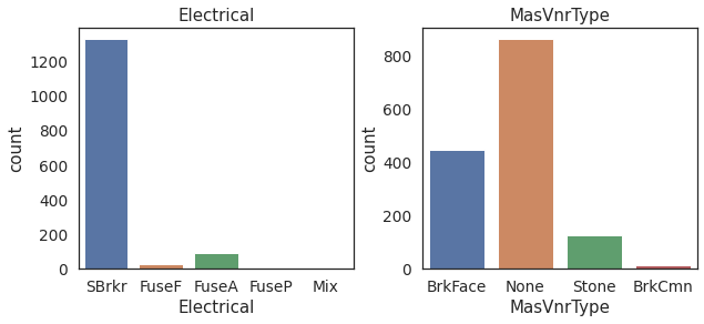
SBrkr is the most frequent category in the Electrical.
None is the most frequent category in MasVnrType.
Impute the missing categories with most frequently occuring ones.
cat_mode_mapper = housing[FEATURES['cat']].mode().iloc[0].to_dict()

def impute_cat(X,feat_to_mode=['Electrical','MasVnrType'], mapper = cat_mode_mapper):
    """
    Imputes missing values in Electrical and MasVnrType with modes,
    and replaces NaN values in all other categorical features with 'Missing'
    """
    for col, mode in mapper.items():
        if col in feat_to_mode:
            X[col].fillna(mode,inplace=True)
        else:
            X[col].fillna('Missing',inplace=True)
    return X

cat_Imputer = FunctionTransformer(impute_cat,validate=False,
                                      kw_args=dict(feat_to_mode=['Electrical','MasVnrType'],
                                                   mapper=cat_mode_mapper))
cat_Imputer.fit(housing)
transformers.append(('cat_Imputer',cat_Imputer))
housing = cat_Imputer.transform(housing)
# Check if there are missing values in the categorical features any more
housing[FEATURES['cat']].isnull().sum()
MSSubClass       0
MSZoning         0
Street           0
Alley            0
LotShape         0
LandContour      0
Utilities        0
LotConfig        0
LandSlope        0
Neighborhood     0
Condition1       0
Condition2       0
BldgType         0
HouseStyle       0
RoofStyle        0
RoofMatl         0
Exterior1st      0
Exterior2nd      0
MasVnrType       0
ExterQual        0
ExterCond        0
Foundation       0
BsmtQual         0
BsmtCond         0
BsmtExposure     0
BsmtFinType1     0
BsmtFinType2     0
Heating          0
HeatingQC        0
CentralAir       0
Electrical       0
KitchenQual      0
Functional       0
FireplaceQu      0
GarageType       0
GarageFinish     0
GarageQual       0
GarageCond       0
PavedDrive       0
PoolQC           0
Fence            0
MiscFeature      0
SaleType         0
SaleCondition    0
dtype: int64
1.4.2. Numerical Features
missing_vals_num = pd.DataFrame(columns=['Feature','# of missing values','% of missing values'])
for feature, numNan in housing.isnull().sum().iteritems():
    if housing[feature].dtypes!= 'object' and 'SalePrice' not in feature:
        FEATURES['num'].append(feature)
        if numNan != 0:
            missing_vals_num = pd.concat([missing_vals_num,
                                          pd.DataFrame([feature,numNan,
                                                        (numNan/housing.shape[0])*100],
                                                       index=['Feature','# of missing values','% of missing values']).T])

missing_vals_num.reset_index(drop = True).sort_values(by='# of missing values',ascending=False)
| Feature | # of missing values | % of missing values | |
|---|---|---|---|
| 0 | LotFrontage | 256 | 17.6066 |
| 2 | GarageYrBlt | 81 | 5.57084 |
| 1 | MasVnrArea | 8 | 0.550206 |
1.4.2.1. MasVnrArea
MasVnrArea: Since the most common category (None) was imputed for the missing values in the cat feature, MasVnrType, it will make sense to impute missing values in MasVnrArea with median MasVnrArea value of houses that have “None” as the MasVnrType.
MedianMasVnrArea = housing[housing['MasVnrType'] == 'None']['MasVnrArea'].median()
print("Median MasVnrArea: ",MedianMasVnrArea)
Median MasVnrArea: 0.0
1.4.2.2. GarageYrBlt
GarageYrBlt: these are same rows which have missing values in other garage related features, indicating that these houses do not have a garage. Imputing median value is a safe option, as these houses have already been flagged as missing a garage in the categorical features.
MedianGarageYrBlt = housing['GarageYrBlt'].median()
print("Median GarageYrBlt: ",MedianGarageYrBlt)
Median GarageYrBlt: 1980.0
1.4.2.3. LotForntage
LotForntage: missing values needs to be handled more carefully as they amount to 17.73% of the total oberservation.
Let’s take a look at the other three features associated with Lot: LotConfig, LotShape, and LotArea
plt.figure(figsize = (15,5))
plt.subplots_adjust(wspace=0.25)
plt.subplot(1,2,1)
sns.boxplot(x='LotConfig',y='LotFrontage',data=housing,hue='LotShape')
plt.subplot(1,2,2)
sns.scatterplot(x='LotArea',y='LotFrontage',data=housing,marker='s',alpha=0.25)
<matplotlib.axes._subplots.AxesSubplot at 0x7f475d537f60>
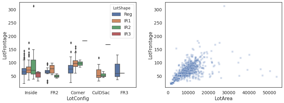
Group the data by LotShape and LotConfig and compute group specific median LotFrontage.
Impute missing LotFrontage with group specific median LotFrontage values.
num_median_mapper = housing[FEATURES['num']].median().to_dict()
num_median_mapper['LotFrontage'] = housing.groupby(['LotConfig','LotShape'])['LotFrontage'].median().to_dict()

def impute_num(X,mapper=num_median_mapper):
    for feat,vals in mapper.items():
        if feat == 'LotFrontage':
            for key,val in vals.items():
                LotConfig,LotShape = key
                X.loc[(X['LotFrontage'].isnull()) & (X['LotConfig']==LotConfig) & (X['LotShape']==LotShape),['LotFrontage']] = val
            X.loc[X['LotFrontage'].isnull(),'LotFrontage'] = X['LotFrontage'].median()
        else:
            X[feat].fillna(vals,inplace=True)
    return X

num_imputer = FunctionTransformer(impute_num,validate=False,
                                      kw_args=dict(mapper=num_median_mapper))
num_imputer.fit(housing)

transformers.append(('num_imputer',num_imputer))

housing = num_imputer.transform(housing)
# Check if there are any missing values in the entire dataset anymore.
housing.isnull().sum().sum()
0
Data cleaning is done at this point.
Next, we will add more data to the dataset from other sources.
1.5. Data Augmentation
In this part, we will add more features to the dataset by gathering data from other sources like Google’s Geocoding API and uszipcode library.
# Number of unique categories per categorical feature
unique_cats = defaultdict(int)

for col in housing.columns:
    if housing[col].dtypes == 'object':
        unique_cats[col] = housing[col].nunique()
        #print('{0}:\t\t {1} unique categories'.format(col,housing_cat[col].nunique()))

num_unique_cats = pd.Series(unique_cats)
num_unique_cats.sort_values(ascending = False)
Neighborhood     25
Exterior2nd      16
MSSubClass       15
Exterior1st      15
Condition1        9
SaleType          9
Condition2        8
HouseStyle        8
RoofMatl          7
GarageType        7
Functional        7
BsmtFinType1      7
BsmtFinType2      7
Heating           6
RoofStyle         6
SaleCondition     6
Foundation        6
FireplaceQu       6
GarageCond        6
GarageQual        6
MSZoning          5
LotConfig         5
MiscFeature       5
Fence             5
BldgType          5
HeatingQC         5
ExterCond         5
Electrical        5
BsmtQual          5
BsmtCond          5
BsmtExposure      5
MasVnrType        4
LotShape          4
ExterQual         4
KitchenQual       4
PoolQC            4
GarageFinish      4
LandContour       4
Alley             3
LandSlope         3
PavedDrive        3
Utilities         2
Street            2
CentralAir        2
dtype: int64
Neighborhood has most number of unique categories. The categories are some sort of location names.
1.5.1. Google API: Geocoding
In this section, we will extract Latitude and Longitude coordinates, and zipcodes from Google’s Geocoding API.
import googlemaps
import json
# Import the googlemaps API key
with open('data/keys.json') as file:
    keys = json.load(file)

gmaps = googlemaps.Client(key=keys['geocoding'])
# List of neighborhoods
housing.Neighborhood.unique()
array(['CollgCr', 'Veenker', 'Crawfor', 'NoRidge', 'Mitchel', 'Somerst',
       'NWAmes', 'OldTown', 'BrkSide', 'Sawyer', 'NridgHt', 'NAmes',
       'SawyerW', 'IDOTRR', 'MeadowV', 'Edwards', 'Timber', 'Gilbert',
       'StoneBr', 'ClearCr', 'NPkVill', 'Blmngtn', 'BrDale', 'SWISU',
       'Blueste'], dtype=object)
neighborhoods = {"CollgCr":"College Creek","Veenker":"Veenker",
                 "Crawfor":"Crawford","NoRidge":"Northridge",
                 "Mitchel":"Mitchell","Somerst":"Somerset",
                 "NWAmes":"Northwest Ames","OldTown":"Old Town",
                 "BrkSide":"Brookside","Sawyer":"Sawyer",
                 "NridgHt":"Northridge Heights","NAmes":"North Ames",
                 "SawyerW":"Sawyer West","IDOTRR":"Iowa DOT and Rail Road",
                 "MeadowV":"Meadow Village","Edwards":"Edwards",
                 "Timber":"Timberland","Gilbert":"Gilbert",
                 "StoneBr":"Stone Brook","ClearCr":"Clear Creek",
                 "NPkVill":"Northpark Villa","Blmngtn":"Bloomington Heights",
                 "BrDale":"Briardale","SWISU":"South & West of Iowa State University",
                 "Blueste":"Bluestem"}
Let’s create a separate dataframe with unique Neighborhood categories
geo_df = pd.DataFrame(housing.Neighborhood.unique(),columns=['Neighborhood'])
geo_df.head()
| Neighborhood | |
|---|---|
| 0 | CollgCr |
| 1 | Veenker |
| 2 | Crawfor |
| 3 | NoRidge |
| 4 | Mitchel |
import re
def getGeoInfo(Neighborhood, output):
    '''
     Enter the Neighborhood and the kind of output you want (lat,lng, or zipcode)
    '''
    def getZipCode(formatted_address):
        substr = re.findall('IA \d{5}, USA',formatted_address)
        if len(substr) == 0:
            return 'Missing'
        else:
            return re.findall('\d{5}',substr[0])[0]

    geocode_result = gmaps.geocode(neighborhoods[Neighborhood]+', Ames, IA')

    i = 0
    while True:
        if i == len(geocode_result):
            idx = None
            break
        elif 'IA' in geocode_result[i]['formatted_address']:
            idx = i
            break
        i += 1

    lat = geocode_result[idx]['geometry']['location']['lat']
    lng = geocode_result[idx]['geometry']['location']['lng']
    zipcode = getZipCode(geocode_result[idx]['formatted_address'])

    if output == 'lat':
        return lat
    elif output == 'lng':
        return lng
    elif output == 'zipcode':
        return zipcode
    else:
        return 'invalid output!'
geo_df['Lat'] = geo_df['Neighborhood'].apply(getGeoInfo,output='lat')
geo_df['Lng'] = geo_df['Neighborhood'].apply(getGeoInfo,output='lng')
geo_df['zipcode'] = geo_df['Neighborhood'].apply(getGeoInfo,output='zipcode')
geo_df
| Neighborhood | Lat | Lng | zipcode | |
|---|---|---|---|---|
| 0 | CollgCr | 42.022197 | -93.651510 | Missing |
| 1 | Veenker | 42.041304 | -93.650302 | 50011 |
| 2 | Crawfor | 42.018614 | -93.648898 | 50014 |
| 3 | NoRidge | 42.047831 | -93.646745 | 50010 |
| 4 | Mitchel | 41.990308 | -93.601053 | 50010 |
| 5 | Somerst | 42.052628 | -93.644582 | 50010 |
| 6 | NWAmes | 42.038277 | -93.625770 | 50010 |
| 7 | OldTown | 42.029046 | -93.614340 | 50010 |
| 8 | BrkSide | 42.028653 | -93.630386 | 50010 |
| 9 | Sawyer | 42.033903 | -93.677066 | 50014 |
| 10 | NridgHt | 42.059773 | -93.649471 | 50010 |
| 11 | NAmes | 42.049358 | -93.622442 | 50010 |
| 12 | SawyerW | 42.024906 | -93.659599 | 50014 |
| 13 | IDOTRR | 42.021997 | -93.622018 | 50010 |
| 14 | MeadowV | 41.992448 | -93.602645 | 50010 |
| 15 | Edwards | 42.015510 | -93.685391 | 50014 |
| 16 | Timber | 41.999973 | -93.649693 | 50014 |
| 17 | Gilbert | 42.106929 | -93.649663 | 50105 |
| 18 | StoneBr | 42.059727 | -93.637642 | 50010 |
| 19 | ClearCr | 42.036097 | -93.648830 | 50011 |
| 20 | NPkVill | 42.030781 | -93.631913 | Missing |
| 21 | Blmngtn | 42.056376 | -93.644471 | 50010 |
| 22 | BrDale | 42.052795 | -93.628821 | 50010 |
| 23 | SWISU | 42.026657 | -93.646452 | 50011 |
| 24 | Blueste | 42.023090 | -93.663783 | 50014 |
In geo_df, there are two Neighborhoods (CollgCr, NPkVill) for which Google’s gecoding API was not able to provide the zipcode.
Lets look at Lat vs. Lng scatter plot to see which neighborhoods are close to those with missing zipcode.
sns.scatterplot(x='Lat',y='Lng',
                data=geo_df,
                hue='zipcode',
                palette=['red','cyan','magenta','green','blue'],
                alpha=1,s=100)
plt.legend(loc='center right',bbox_to_anchor = (1.35,0.5))
_=plt.xticks(rotation=45)
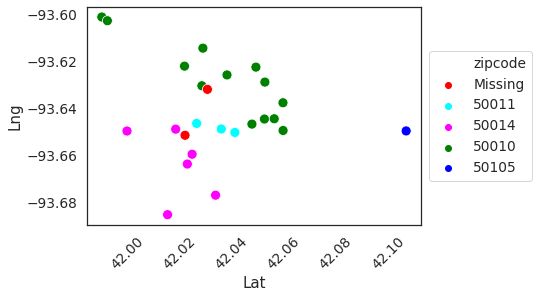
It will be reasonable to impute missing zipcodes with the closest neighbors, but there is another library that can provide zipcode info based on geo coordinates.
It is the uszipcode library https://pypi.org/project/uszipcode/
This library can be used to extract demographic information of different locations in US.
1.5.2. uszipcode
In this section, we will impute the missing zipcode, as well as augment our dataset with more features like popution density, total population, median household income, total number of housing units, etc.
from uszipcode import SearchEngine
def getMoreFeat(a,b):
    '''
    Can take zipcode or [lat,lng] as inputs (a) and return requested information about location,
    The information requested should be specifed as the second argument (b).

    Acceptable requests are:'lat', 'lng',
                            'population', 'zipcode',
                            'population_density','housing_units',
                            'occupied_housing_units', 'median_home_value'
                            'median_household_income'

    '''
    def getZipCode(a):
        geo_info = search.by_coordinates(a[0],a[1],radius=5)
        i = 0
        while True:
            if i == len(geo_info):
                idx = None
                break
            elif (geo_info[i].post_office_city == 'Ames, IA') and (geo_info[i].major_city == 'Ames') and (geo_info[i].common_city_list[0] == 'Ames'):
                idx = i
                break
            i += 1

        if idx == None:
            print("Coordinates don't belong to Ames, IA. NaN returned")
            return np.nan
        else:
            return geo_info[idx].to_dict()[b]

    def getRequest(zipcode,b):
        geo_info = search.by_zipcode(zipcode)
        return geo_info.to_dict()[b]


    search = SearchEngine(simple_zipcode=True)

    if b == 'zipcode':
        return getZipCode(a)
    elif b in ['lat', 'lng', 'population', 'zipcode',
                  'population_density','housing_units',
                  'occupied_housing_units', 'median_home_value',
                  'median_household_income']:
        return getRequest(a,b)
geo_df.loc[geo_df.zipcode=='Missing','zipcode'] = geo_df.loc[geo_df.zipcode=='Missing',['Lat','Lng']].apply(getMoreFeat,axis=1,b='zipcode')
geo_df['median_household_income'] = geo_df['zipcode'].apply(getMoreFeat,b='median_household_income')
geo_df['median_home_value'] = geo_df['zipcode'].apply(getMoreFeat,b='median_home_value')
geo_df
| Neighborhood | Lat | Lng | zipcode | median_household_income | median_home_value | |
|---|---|---|---|---|---|---|
| 0 | CollgCr | 42.022197 | -93.651510 | 50010 | 48189.0 | 165300.0 |
| 1 | Veenker | 42.041304 | -93.650302 | 50011 | NaN | NaN |
| 2 | Crawfor | 42.018614 | -93.648898 | 50014 | 37661.0 | 212500.0 |
| 3 | NoRidge | 42.047831 | -93.646745 | 50010 | 48189.0 | 165300.0 |
| 4 | Mitchel | 41.990308 | -93.601053 | 50010 | 48189.0 | 165300.0 |
| 5 | Somerst | 42.052628 | -93.644582 | 50010 | 48189.0 | 165300.0 |
| 6 | NWAmes | 42.038277 | -93.625770 | 50010 | 48189.0 | 165300.0 |
| 7 | OldTown | 42.029046 | -93.614340 | 50010 | 48189.0 | 165300.0 |
| 8 | BrkSide | 42.028653 | -93.630386 | 50010 | 48189.0 | 165300.0 |
| 9 | Sawyer | 42.033903 | -93.677066 | 50014 | 37661.0 | 212500.0 |
| 10 | NridgHt | 42.059773 | -93.649471 | 50010 | 48189.0 | 165300.0 |
| 11 | NAmes | 42.049358 | -93.622442 | 50010 | 48189.0 | 165300.0 |
| 12 | SawyerW | 42.024906 | -93.659599 | 50014 | 37661.0 | 212500.0 |
| 13 | IDOTRR | 42.021997 | -93.622018 | 50010 | 48189.0 | 165300.0 |
| 14 | MeadowV | 41.992448 | -93.602645 | 50010 | 48189.0 | 165300.0 |
| 15 | Edwards | 42.015510 | -93.685391 | 50014 | 37661.0 | 212500.0 |
| 16 | Timber | 41.999973 | -93.649693 | 50014 | 37661.0 | 212500.0 |
| 17 | Gilbert | 42.106929 | -93.649663 | 50105 | 80703.0 | 165400.0 |
| 18 | StoneBr | 42.059727 | -93.637642 | 50010 | 48189.0 | 165300.0 |
| 19 | ClearCr | 42.036097 | -93.648830 | 50011 | NaN | NaN |
| 20 | NPkVill | 42.030781 | -93.631913 | 50010 | 48189.0 | 165300.0 |
| 21 | Blmngtn | 42.056376 | -93.644471 | 50010 | 48189.0 | 165300.0 |
| 22 | BrDale | 42.052795 | -93.628821 | 50010 | 48189.0 | 165300.0 |
| 23 | SWISU | 42.026657 | -93.646452 | 50011 | NaN | NaN |
| 24 | Blueste | 42.023090 | -93.663783 | 50014 | 37661.0 | 212500.0 |
There are missing values in median_household_income and median_home_value column.
Lets impute missing values with most frequently occuring values.
geo_df['zipcode'] = geo_df.zipcode.astype(int)
geo_df.set_index('Neighborhood',inplace=True)

from sklearn.impute import SimpleImputer
imputer = SimpleImputer(strategy='most_frequent')
geo_df = pd.DataFrame(imputer.fit_transform(geo_df),columns=geo_df.columns,index=geo_df.index)

geo_df.reset_index(inplace=True)
geo_df
| Neighborhood | Lat | Lng | zipcode | median_household_income | median_home_value | |
|---|---|---|---|---|---|---|
| 0 | CollgCr | 42.022197 | -93.651510 | 50010.0 | 48189.0 | 165300.0 |
| 1 | Veenker | 42.041304 | -93.650302 | 50011.0 | 48189.0 | 165300.0 |
| 2 | Crawfor | 42.018614 | -93.648898 | 50014.0 | 37661.0 | 212500.0 |
| 3 | NoRidge | 42.047831 | -93.646745 | 50010.0 | 48189.0 | 165300.0 |
| 4 | Mitchel | 41.990308 | -93.601053 | 50010.0 | 48189.0 | 165300.0 |
| 5 | Somerst | 42.052628 | -93.644582 | 50010.0 | 48189.0 | 165300.0 |
| 6 | NWAmes | 42.038277 | -93.625770 | 50010.0 | 48189.0 | 165300.0 |
| 7 | OldTown | 42.029046 | -93.614340 | 50010.0 | 48189.0 | 165300.0 |
| 8 | BrkSide | 42.028653 | -93.630386 | 50010.0 | 48189.0 | 165300.0 |
| 9 | Sawyer | 42.033903 | -93.677066 | 50014.0 | 37661.0 | 212500.0 |
| 10 | NridgHt | 42.059773 | -93.649471 | 50010.0 | 48189.0 | 165300.0 |
| 11 | NAmes | 42.049358 | -93.622442 | 50010.0 | 48189.0 | 165300.0 |
| 12 | SawyerW | 42.024906 | -93.659599 | 50014.0 | 37661.0 | 212500.0 |
| 13 | IDOTRR | 42.021997 | -93.622018 | 50010.0 | 48189.0 | 165300.0 |
| 14 | MeadowV | 41.992448 | -93.602645 | 50010.0 | 48189.0 | 165300.0 |
| 15 | Edwards | 42.015510 | -93.685391 | 50014.0 | 37661.0 | 212500.0 |
| 16 | Timber | 41.999973 | -93.649693 | 50014.0 | 37661.0 | 212500.0 |
| 17 | Gilbert | 42.106929 | -93.649663 | 50105.0 | 80703.0 | 165400.0 |
| 18 | StoneBr | 42.059727 | -93.637642 | 50010.0 | 48189.0 | 165300.0 |
| 19 | ClearCr | 42.036097 | -93.648830 | 50011.0 | 48189.0 | 165300.0 |
| 20 | NPkVill | 42.030781 | -93.631913 | 50010.0 | 48189.0 | 165300.0 |
| 21 | Blmngtn | 42.056376 | -93.644471 | 50010.0 | 48189.0 | 165300.0 |
| 22 | BrDale | 42.052795 | -93.628821 | 50010.0 | 48189.0 | 165300.0 |
| 23 | SWISU | 42.026657 | -93.646452 | 50011.0 | 48189.0 | 165300.0 |
| 24 | Blueste | 42.023090 | -93.663783 | 50014.0 | 37661.0 | 212500.0 |
geo_df.info()
<class 'pandas.core.frame.DataFrame'>
RangeIndex: 25 entries, 0 to 24
Data columns (total 6 columns):
 #   Column                   Non-Null Count  Dtype
---  ------                   --------------  -----
 0   Neighborhood             25 non-null     object
 1   Lat                      25 non-null     float64
 2   Lng                      25 non-null     float64
 3   zipcode                  25 non-null     float64
 4   median_household_income  25 non-null     float64
 5   median_home_value        25 non-null     float64
dtypes: float64(5), object(1)
memory usage: 1.3+ KB
##Adding new features to FEATURES dictionary
for col in geo_df:
    if col == 'Neighborhood':
        print(col+' already in FETAURES["cat"]')
    elif geo_df[col].dtypes == 'object':
        FEATURES['aug_cat'].append(col)
    else:
        FEATURES['aug_num'].append(col)
Neighborhood already in FETAURES["cat"]
Now that geo_df is ready, which includes geographical and demographical information, lets merge it with the main dataset.
def augment(X,geo_df):
    X.reset_index(inplace=True)
    X = X.merge(geo_df,how='left')
    X.set_index('Id',inplace=True)
    return X

augmenter = FunctionTransformer(augment,validate=False,kw_args=dict(geo_df=geo_df))
transformers.append(('augmenter',augmenter))

housing = augmenter.fit_transform(housing)
print(housing.shape)
(1454, 87)
test = pd.read_csv('data/test.csv',index_col='Id')
my_pipeline = Pipeline(transformers)
my_pipeline.fit(housing_raw)
housing_temp = my_pipeline.transform(housing_raw)

print('Manually and pipeline created datasets are equal:')
print(housing.drop('log1p(SalePrice)',axis=1).equals(housing_temp))

test_temp = my_pipeline.transform(test)
Manually and pipeline created datasets are equal:
True
# Add newly added numerical features to FEATURES dictionary
for feature in housing.columns:
    if feature not in FEATURES['cat']+FEATURES['num']+FEATURES['aug_num']:
        print(feature+' is missing in housing_temp')
SalePrice is missing in housing_temp
log1p(SalePrice) is missing in housing_temp
Correlations of the newly added geographic and demograpic features with the target variable.
plt.figure(figsize=(6,4))
sns.heatmap(housing[['log1p(SalePrice)','SalePrice','Lat','Lng','zipcode','median_household_income','median_home_value']].corr(),
           vmin=-1,vmax=1,cmap='coolwarm',annot=True,annot_kws=dict(size=12),fmt='.2f')
plt.title('Correlation Matrix')
Text(0.5, 1.0, 'Correlation Matrix')
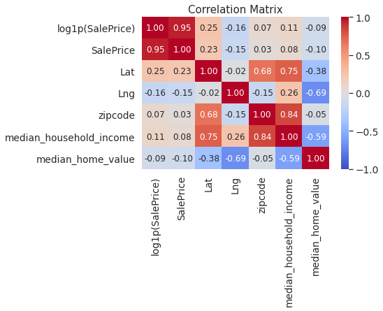
Correlations are high, but lets keep these features for now. We will come back to this later.
print('Dimensions of the dataset',housing[FEATURES['num']+FEATURES['cat']+FEATURES['aug_num']].shape)
Dimensions of the dataset (1454, 85)
At this point, data is free of outliers and missing values.
with open('data/wrangled_data.pkl','wb') as file:
    pickle.dump((housing,FEATURES,transformers),file)